
Section 2.6 Timing characteristics of logic circuits
An ideal gate represents a truth table, which is simply an input-output relationship. The output is presumed to change simultaneously with a causative change in an input. In an actual logic circuit, however, the output changes a brief time after the input changes. This time is called the propagation delay of the circuit. Propagation delay is at the root of what we are talking about when we say a digital system is “fast” or “slow”.
Propagation delay is illustrated in Figure 2.6.1, below. An inverter was wired up on a solderless breadboard with its input driven by a function generator, and its output viewed on an oscilloscope. The small oscillations around the LOW and HIGH voltage levels are typical of real logic circuits, and are within the limits specified by \(V_{IH}\) and \(V_{IL}\) for correct operation. It is evident that the output transitions occur a measurable time after the input transitions.
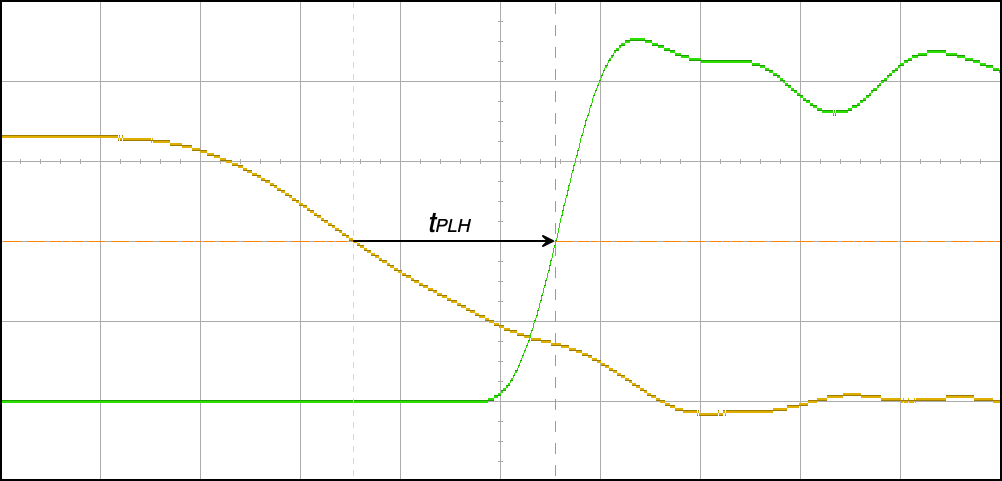
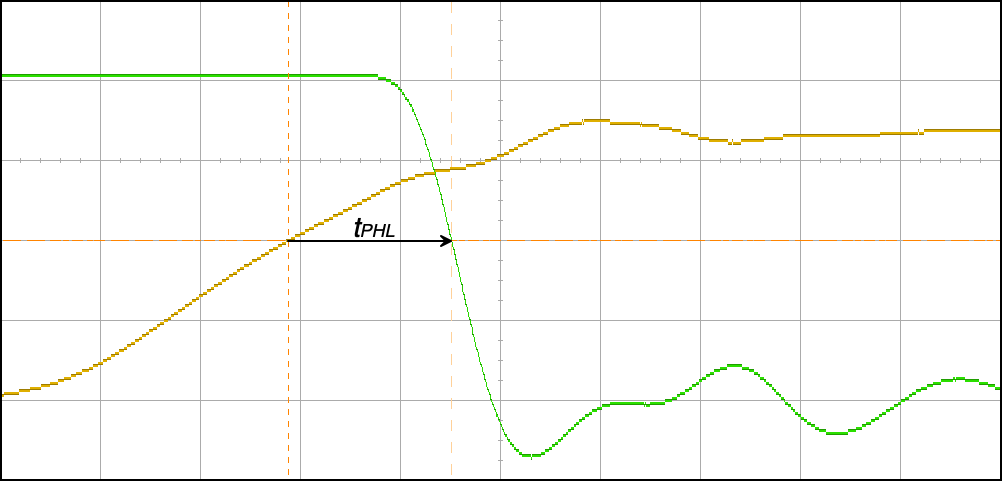
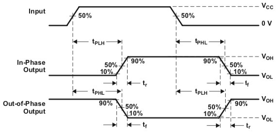
A transition in a signal from LOW to HIGH is called a rising edge or positive edge. A transition from HIGH to LOW is called a falling edge or negative edge. Propagation delays are measured from an edge of the input to the next edge of the output, as shown in Figure 2.6.2. The delay from an input edge of either polarity to a rising edge at the output is called \(t_{PLH}\) (LOW-to-HIGH). If the output edge is falling, the delay is called \(t_{PHL}\) (HIGH-to-LOW). The designation of a delay as \(t_{PLH}\) or \(t_{PHL}\) depends only on the polarity of the output edge.
Propagation delays are defined between particular points on the rising or falling edges. For LS-series devices, they are measured between the point where the input crosses 1.3V and the point where the output crosses 1.3V. For the HC-series CMOS family, delays are measured between the points where input and output cross \(V_{DD}/2\) (in Figure 2.6.1. the supply voltage is 4V and the threshold is 2V). Other logic families may define these reference points in yet other ways, so always check the datasheet.
Typical and maximum (worst case) values for propagation delay are tabulated in datasheets (for example, Figure 2.6.3). Sometimes, no distinction is made between \(t_{PLH}\) and \(t_{PHL}\text{,}\) and the delay is denoted by a single symbol such as \(t_{d}\text{,}\) \(t_{p}\text{,}\) or \(t_{pd}\text{.}\) According to the table in Figure 2.6.3, propagation delay depends on the supply voltage, \(V_{CC}\text{.}\) The typical values for \(t_{PLH}\) and \(t_{PHL}\) are about 9ns for the conditions (\(V_{CC}=4\)V) used for the measurements in Figure 2.6.1. The measured values, 8ns and 10ns, are within the typical range for this device, according to the datasheet.
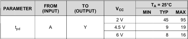
The propagation delay for a circuit consisting of one gate driving another is the sum of their individual propagation delays. For a combination of two HC04 inverters, the typical delay would be 18ns, and the maximum (worst case) delay would be 38ns.
Propagation delays in a circuit are a combination of logic delays, related to how fast a transistor can switch between ON and OFF, and wire delays, which are the time required for a signal to propagate from gate to gate within an integrated circuit, and from package to package on a circuit board. The velocity of propagation on a wire is less than the speed of light, and can be measured in the lab.
The physical origins of logic delays and wire delays are beyond the scope of this course, but may be understood using physical principles covered in Phys 14 and Engs 22. Sections 4.2 and 5.1 of Reference [2] provide more details for the interested reader.

