Any combinational logic function is completely described by a truth table. From there, we have seen how logic equations may be derived, minimized, and finally implemented as gate-level circuits. When integrated circuits contained only small numbers of gates (see Section 1.6), even a system of modest complexity could require a large number of packages and a correspondingly large circuit board. In response, designers searched for other ways to implement logic at higher levels of integration.
One clever discovery was that a four-to-one multiplexer could be used to implement any function of two variables. Recall that the logic equation for a four-to-one multiplexer is:
\begin{equation*}
y = S_1^\prime S_0^\prime A + S_1^\prime S_0 B + S_1 S_0^\prime C + S_1 S_0 D
\end{equation*}
Each term contains one of the four possible combinations of the select bits \(S_1\) and \(S_0\text{.}\) The remaining inputs \(A\) through \(D\) are used to select which combinations will yield a TRUE output. For example, to implement \(y = S_1^\prime S_0 + S_1 S_0^\prime\text{,}\) you would wire inputs \(A\) and \(D\) to ’0’, and inputs \(B\) and \(C\) to ’1’. An eight-to-one multiplexer could be wired to implement any function of three variables, and a sixteen-to-one multiplexer could be wired to implement any function of four variables. If you are counting transistors, this may not compare favorably with a minimum sum-of-products constructed from individual gates. But, if the individual gates require several packages on a circuit board, and the equivalent multiplexer circuit can be built with only one package, you save on area and maybe power and speed as well.
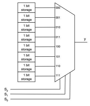
This is an old idea, that, surprisingly, lives on in the programmable logic devices used in this course (see Section 11.1). Figure 4.5.1 shows an eight-to-one multiplexer, with each input connected to a small block of logic that can be programmed to store either ’1’ or ’0’ (we’ll learn about these in a future chapter). The combination of storage and multiplexer is called a lookup table, or LUT. (This isn’t exactly how they are made, but it is a very convenient model.) Depending on the programming, the LUT can implement any function of three variables. Contemporary programmable devices contain thousands of small LUTs, each with as many as six inputs. Rather than changing the gates and wiring of a gate-level circuit to modify a function, one may simply change the programming of its LUT.
Figure4.5.1.Model of a three-input lookup table (LUT) as eight bits of storage and an 8-to-1 multiplexer. The LUT can store the truth table for any function of three logic variables, \(Y = f(S_2, S_1, S_0)\text{.}\)
Checkpoint4.5.2.
What logic function is implemented by the LUT in Figure 4.5.1, if the stored bits are (read from top to bottom), \(1, \, 1, \, 0, \, 0, \, 0, \, 1, \, 0, \, 1\text{?}\)